Repeated Cross-Validation for cv.glmnet

This functions returns the best lambda of repeated glmnet::cv.glmnet() calls.

rcv.glmnet(
    x, y,
    lambda = NULL,
    nrepcv = 100L, nfolds = 10L,
    ...,
    trace.it = interactive(), mc.cores = getOption("mc.cores", 1L)
)

Arguments

x	matrix, as in cv.glmnet.
y	response as in cv.glmnet.
lambda	numeric, optional user-supplied lambda sequence; default is NULL and glmnet chooeses its own sequence.
nrepcv	integer(1), number of repeated cross-validations (outer loop).
nfolds	integer, number of folds, same as in cv.glmnet.
...	further arguments passed to cv.glmnet.
trace.it	integer, if trace.it = 1, then a progress bar is displayed.
mc.cores	integer, number of cores used for parallelisation.

Value

An object of class rcv.glmnet that extends the cv.glmnet class.

References

Jerome Friedman, Trevor Hastie, Robert Tibshirani (2010). Regularization Paths for Generalized Linear Models via Coordinate Descent. Journal of Statistical Software, 33(1), 1-22. URL https://www.jstatsoft.org/v33/i01/.

Noah Simon, Jerome Friedman, Trevor Hastie, Rob Tibshirani (2011). Regularization Paths for Cox's Proportional Hazards Model via Coordinate Descent. Journal of Statistical Software, 39(5), 1-13. URL https://www.jstatsoft.org/v39/i05/.

See also

glmnet::cv.glmnet()

Author

Sebastian Gibb

Examples

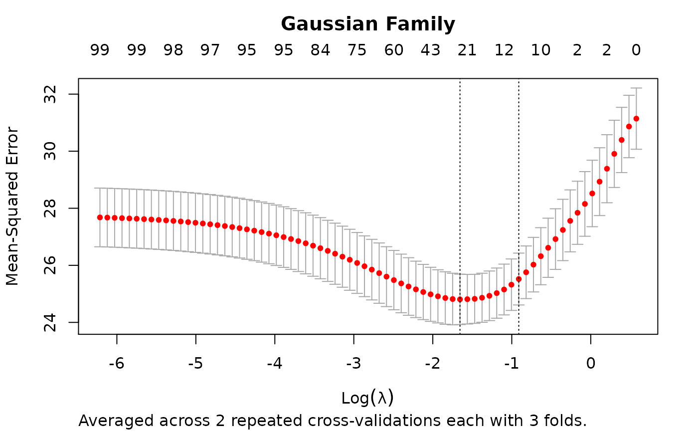
# Examples taken from ?"glmnet::cv.glmnet"
set.seed(1010)
n <- 1000
p <- 100
nzc <- trunc(p/10)
x <- matrix(rnorm(n * p), n, p)
beta <- rnorm(nzc)
fx <- x[, seq(nzc)] %*% beta
eps <- rnorm(n) * 5
y <- drop(fx + eps)
set.seed(1011)
# nrepcv should usually be higher but to keep the runtime of the example low
# we choose 2 here
rcvob <- rcv.glmnet(x, y, nrepcv = 2, nfolds = 3)
plot(rcvob)
title("Gaussian Family", line = 2.5)
coef(rcvob)
#> 101 x 1 sparse Matrix of class "dgCMatrix"
#>                      1
#> (Intercept) -0.1162737
#> V1          -0.2171531
#> V2           0.3237422
#> V3           .        
#> V4          -0.2190339
#> V5          -0.1856601
#> V6           0.2530652
#> V7           0.1874832
#> V8          -1.3574323
#> V9           1.0162046
#> V10          0.1558299
#> V11          .        
#> V12          .        
#> V13          .        
#> V14          .        
#> V15          .        
#> V16          .        
#> V17          .        
#> V18          .        
#> V19          .        
#> V20          .        
#> V21          .        
#> V22          .        
#> V23          .        
#> V24          .        
#> V25          .        
#> V26          .        
#> V27          .        
#> V28          .        
#> V29          .        
#> V30          .        
#> V31          .        
#> V32          .        
#> V33          .        
#> V34          .        
#> V35          .        
#> V36          .        
#> V37          .        
#> V38          .        
#> V39          .        
#> V40          .        
#> V41          .        
#> V42          .        
#> V43          .        
#> V44          .        
#> V45          .        
#> V46          .        
#> V47          .        
#> V48          .        
#> V49          .        
#> V50          .        
#> V51          .        
#> V52          .        
#> V53          .        
#> V54          .        
#> V55          .        
#> V56          .        
#> V57          .        
#> V58          .        
#> V59          .        
#> V60          .        
#> V61          .        
#> V62          .        
#> V63          .        
#> V64          .        
#> V65          .        
#> V66          .        
#> V67          .        
#> V68          .        
#> V69          .        
#> V70          .        
#> V71          .        
#> V72          .        
#> V73          .        
#> V74          .        
#> V75         -0.1420966
#> V76          .        
#> V77          .        
#> V78          .        
#> V79          .        
#> V80          .        
#> V81          .        
#> V82          .        
#> V83          .        
#> V84          .        
#> V85          .        
#> V86          .        
#> V87          .        
#> V88          .        
#> V89          .        
#> V90          .        
#> V91          .        
#> V92          .        
#> V93          .        
#> V94          .        
#> V95          .        
#> V96          .        
#> V97          .        
#> V98          .        
#> V99          .        
#> V100         .        
predict(rcvob, newx = x[1:5, ], s = "lambda.min")
#>               1
#> [1,] -1.3447658
#> [2,]  0.9443441
#> [3,]  0.6989746
#> [4,]  1.8698290
#> [5,] -4.7372693