A new machine-learning-based prediction of survival in patients with end-stage liver disease
Supplement
Sebastian Gibb1
Thomas Berg
Adam Herber
Berend Isermann
Thorsten Kaiser
Last updated: 2022-12-05
Checks: 7 0
Knit directory:
ampel-leipzig-meld/
This reproducible R Markdown analysis was created with workflowr (version 1.7.0). The Checks tab describes the reproducibility checks that were applied when the results were created. The Past versions tab lists the development history.
Great! Since the R Markdown file has been committed to the Git repository, you know the exact version of the code that produced these results.
Great job! The global environment was empty. Objects defined in the global environment can affect the analysis in your R Markdown file in unknown ways. For reproduciblity it’s best to always run the code in an empty environment.
The command set.seed(20210604) was run prior to running the code in the R Markdown file.
Setting a seed ensures that any results that rely on randomness, e.g.
subsampling or permutations, are reproducible.
Great job! Recording the operating system, R version, and package versions is critical for reproducibility.
Nice! There were no cached chunks for this analysis, so you can be confident that you successfully produced the results during this run.
Great job! Using relative paths to the files within your workflowr project makes it easier to run your code on other machines.
Great! You are using Git for version control. Tracking code development and connecting the code version to the results is critical for reproducibility.
The results in this page were generated with repository version be55dc7. See the Past versions tab to see a history of the changes made to the R Markdown and HTML files.
Note that you need to be careful to ensure that all relevant files for the
analysis have been committed to Git prior to generating the results (you can
use wflow_publish or wflow_git_commit). workflowr only
checks the R Markdown file, but you know if there are other scripts or data
files that it depends on. Below is the status of the Git repository when the
results were generated:
Ignored files:
    Ignored:    _targets/
    Ignored:    analysis/article.md
    Ignored:    container/
    Ignored:    logs/
    Ignored:    scripts/R.sh

Untracked files:
    Untracked:  submission/
Note that any generated files, e.g. HTML, png, CSS, etc., are not included in this status report because it is ok for generated content to have uncommitted changes.
These are the previous versions of the repository in which changes were made
to the R Markdown (analysis/supplement.Rmd) and HTML (docs/supplement.html)
files. If you’ve configured a remote Git repository (see
?wflow_git_remote), click on the hyperlinks in the table below to
view the files as they were in that past version.
| File | Version | Author | Date | Message |
|---|---|---|---|---|
| Rmd | be55dc7 | Sebastian Gibb | 2022-12-05 | feat: add confidence bands to roc plots |
| html | 88f7b9f | Sebastian Gibb | 2022-12-01 | chore: rebuild site |
| Rmd | b4631f6 | Sebastian Gibb | 2022-12-01 | fix: typos |
| html | 5235082 | Sebastian Gibb | 2022-11-30 | chore: rebuild site |
| Rmd | e1aebf7 | Sebastian Gibb | 2022-11-30 | feat: add MELD 3.0 and adapt to reviewer’s suggestions |
| Rmd | fba81f5 | Sebastian Gibb | 2022-11-27 | feat: add MELD 3.0 score |
| Rmd | 95c0de8 | Sebastian Gibb | 2022-11-27 | refactor: change supplemental figure 2.1 according to reviewer’s suggestions |
| html | 1821ea1 | Sebastian Gibb | 2022-08-10 | chore: rebuild site |
| Rmd | 6315aaa | Sebastian Gibb | 2022-08-10 | refactor: drop DS from author list |
| html | 0d43824 | Sebastian Gibb | 2022-08-09 | chore: rebuild site |
| Rmd | bbdb3a2 | Sebastian Gibb | 2022-08-09 | fix: add dash between machine-learning |
| html | 1403bda | Sebastian Gibb | 2022-08-09 | chore: rebuild site |
| Rmd | 849ca09 | Sebastian Gibb | 2022-08-09 | refactor: add additional co-author |
| Rmd | d9f15ae | Sebastian Gibb | 2022-07-23 | fix: typo |
| html | 68ef9aa | Sebastian Gibb | 2022-07-22 | chore: rebuild site |
| Rmd | e6cf8a2 | Sebastian Gibb | 2022-07-22 | refactor: apply proofreading suggestions |
| html | 83e3c7a | Sebastian Gibb | 2022-07-19 | chore: rebuild site |
| Rmd | 8939c2c | Sebastian Gibb | 2022-07-19 | feat: extend supplement with survival plot |
| Rmd | 2155e58 | Sebastian Gibb | 2022-07-19 | refactor: create png and pdf just for non-html output |
| html | 65d58c4 | Sebastian Gibb | 2022-07-18 | chore: rebuild site |
| Rmd | a0f1d2e | Sebastian Gibb | 2022-07-18 | feat: generate png and pdfs for each plot |
| Rmd | 49d8c41 | Sebastian Gibb | 2022-07-18 | chore: suppress code output in supplement |
| Rmd | 9d4a890 | Sebastian Gibb | 2022-07-18 | feat: use 1200 dpi as required by labm for word output |
| html | fb43d01 | Sebastian Gibb | 2022-06-19 | chore: rebuild site |
| html | ebe29cf | Sebastian Gibb | 2022-06-16 | chore: rebuild site |
| Rmd | 2c8fd1a | Sebastian Gibb | 2022-06-15 | refactor: use short journal names |
| html | 8035219 | Sebastian Gibb | 2022-06-15 | chore: rebuild site |
| Rmd | 19d9fed | Sebastian Gibb | 2022-06-15 | feat: further work on the manuscript |
| html | d3e9462 | Sebastian Gibb | 2022-06-06 | chore: rebuild site |
| html | b20484a | Sebastian Gibb | 2022-06-06 | chore: rebuild site |
| Rmd | 01f934b | Sebastian Gibb | 2022-06-06 | feat: add first discussion draft |
| html | 983ec69 | Sebastian Gibb | 2022-03-17 | chore: rebuild site |
| html | 373e7d8 | Sebastian Gibb | 2021-10-20 | chore: rebuild site |
| html | df8964f | Sebastian Gibb | 2021-10-15 | chore: rebuild site |
| html | c66640c | Sebastian Gibb | 2021-09-14 | feat: first nnet tests |
| html | afa48d9 | Sebastian Gibb | 2021-08-07 | chore: rebuild site |
| Rmd | 3957af7 | Sebastian Gibb | 2021-08-02 | refactor: move common yaml headers into _site.yml |
| html | 3aab3e1 | Sebastian Gibb | 2021-08-01 | chore: rebuild site |
| Rmd | 91bfbd2 | Sebastian Gibb | 2021-08-01 | feat: add first article draft with pandoc filters |
1 Survival plot
tar_load(zlog_data)
srv <- Surv(zlog_data$DaysAtRisk, zlog_data$Deceased)
col <- palette.colors(nlevels(zlog_data$MeldCategory))

srvfit <- survfit(srv ~ 1)
times <- c(2, 7, 14, 30, 90)

## calculate risk tables
sm <- summary(srvfit, times = times)
nrisk <- as.matrix(sm$n.risk)
ncumevents <- as.matrix(cumsum(sm$n.event))
rownames(nrisk) <- rownames(ncumevents) <- times

## keep old graphic parameters and restore them afterwards
old.par <- par(no.readonly = TRUE)

layout(matrix(1:3, nrow = 3), height = c(5, 1, 1))
plot_surv(
    srvfit,
    main = "Kaplan-Meier survival estimate to day 90",
    times = times,
    xmax = 90,
    col = col[2],
    cex = 1.2
)
par(mar = c(1.1, 5.1, 1.1, 2.1))
plot_table(
    nrisk, at = times, main = "Number at risk",
    xaxis = FALSE, cex.text = 1, ylabels = FALSE
)
par(mar = c(1.1, 5.1, 1.1, 2.1))
plot_table(
    ncumevents, at = times, main = "Cumulative number of events",
    xaxis = FALSE, cex.text = 1, ylabels = FALSE
)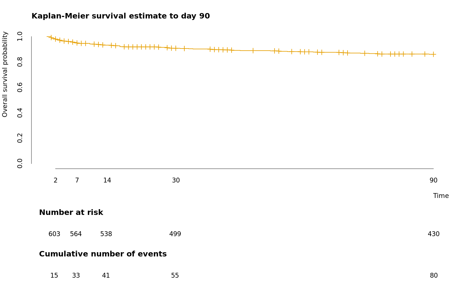
(#fig:survival.plot)Survival plot. Kaplan-Meier survival estimate for the first 90 days of the analyzed population.
| Version | Author | Date |
|---|---|---|
| 83e3c7a | Sebastian Gibb | 2022-07-19 |
par(old.par)2 Benchmark results of machine-learning algorithms
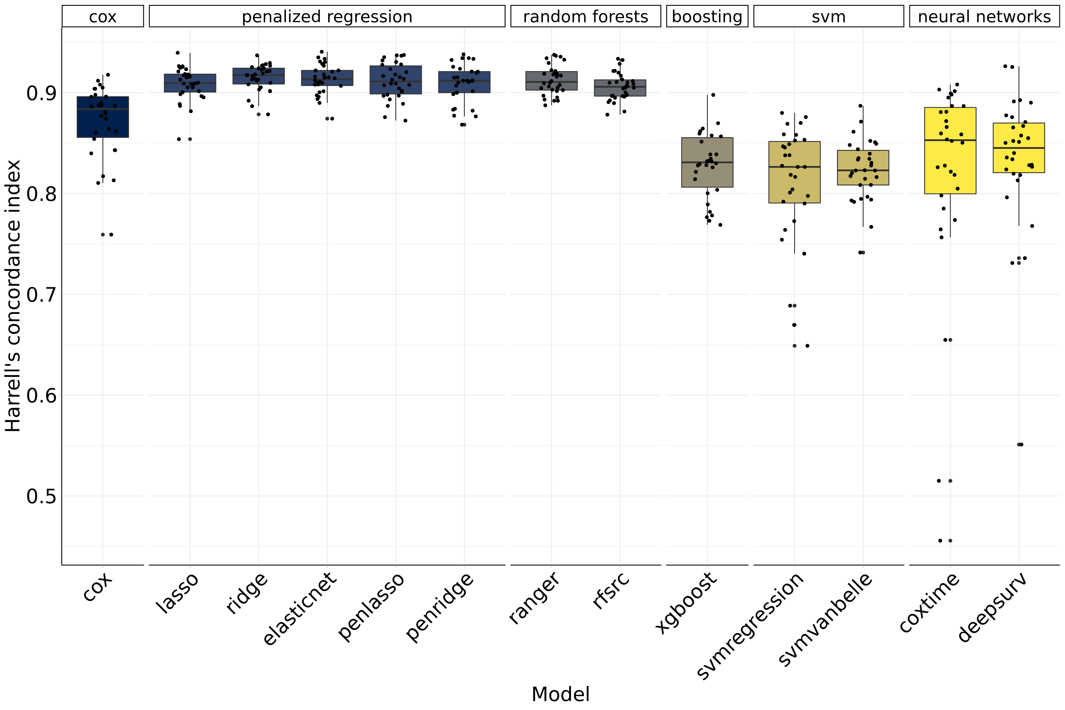
Figure 2.1: Benchmark results of machine-learning algorithms.
| Model | Harrell’s concordance index |
|---|---|
| ridge | 0.915 |
| elasticnet | 0.913 |
| ranger | 0.913 |
| penlasso | 0.911 |
| penridge | 0.909 |
| lasso | 0.909 |
| rfsrc | 0.906 |
| cox | 0.872 |
| deepsurv | 0.833 |
| xgboost | 0.828 |
| svmvanbelle | 0.823 |
| coxtime | 0.819 |
| svmregression | 0.809 |
3 Observed versus MELD-Na-expected 90-day mortality
| MELD category | Observed deaths (n) | Expected deaths (n) | Standardized mortality ratio (SMR) | Observed mortality (%) | Expected mortality (%) |
|---|---|---|---|---|---|
| [6,9] | 1 | 5.8 | 0.2 | 0.5 | 2.8 |
| [10,15) | 4 | 2.9 | 1.4 | 3.0 | 2.3 |
| [15,20) | 5 | 3.1 | 1.6 | 7.5 | 5.1 |
| [20,25) | 15 | 5.7 | 2.6 | 27.1 | 13.0 |
| [25,30) | 22 | 10.2 | 2.1 | 62.5 | 31.1 |
| [30,35) | 14 | 8.1 | 1.7 | 88.0 | 54.2 |
| [35,40) | 9 | 7.5 | 1.2 | 90.0 | 75.1 |
| [40,52) | 6 | 5.1 | 1.2 | 100.0 | 84.4 |
4 ROC curves
![Receiver operating characteristic (ROC) curve. Area under the time-dependent ROC curve (AUC) based on the nonparametric inverse probability of censoring weighting estimate (IPCW) for AMELD, MELD, MELD-Na, MELD 3.0, MELD-Plus7, as described in [@blanche2013]. The dashed lines depict the corresponding 95% confidence bands calculated by threshold averaging as described in [@fawcett2004].](figure/supplement.Rmd/roc-cb-all-1.png)
Figure 4.1: Receiver operating characteristic (ROC) curve. Area under the time-dependent ROC curve (AUC) based on the nonparametric inverse probability of censoring weighting estimate (IPCW) for AMELD, MELD, MELD-Na, MELD 3.0, MELD-Plus7, as described in (Blanche, Dartigues, and Jacqmin-Gadda 2013). The dashed lines depict the corresponding 95% confidence bands calculated by threshold averaging as described in (Fawcett 2004).
![Receiver operating characteristic (ROC) curve. Area under the time-dependent ROC curve (AUC) based on the nonparametric inverse probability of censoring weighting estimate (IPCW) for AMELD, MELD, MELD-Na, MELD 3.0, MELD-Plus7, as described in [@blanche2013]. The dashed lines depict the corresponding 95% confidence bands for AMELD calculated by threshold averaging as described in [@fawcett2004]. The other confidence bands are hidden for easier readability.](figure/supplement.Rmd/roc-cb-ameld-1.png)
Figure 4.2: Receiver operating characteristic (ROC) curve. Area under the time-dependent ROC curve (AUC) based on the nonparametric inverse probability of censoring weighting estimate (IPCW) for AMELD, MELD, MELD-Na, MELD 3.0, MELD-Plus7, as described in (Blanche, Dartigues, and Jacqmin-Gadda 2013). The dashed lines depict the corresponding 95% confidence bands for AMELD calculated by threshold averaging as described in (Fawcett 2004). The other confidence bands are hidden for easier readability.
5 AUROC trend
![Trend in the area under the time-dependent receiver operating characteristic curve (AUROC) based on the nonparametric inverse probability of censoring weighting estimate (IPCW) for AMELD, MELD, MELD-Na, MELD 3.0, and MELD-Plus7, as described in [@blanche2013].](figure/supplement.Rmd/roc-plot-1.png)
Figure 5.1: Trend in the area under the time-dependent receiver operating characteristic curve (AUROC) based on the nonparametric inverse probability of censoring weighting estimate (IPCW) for AMELD, MELD, MELD-Na, MELD 3.0, and MELD-Plus7, as described in (Blanche, Dartigues, and Jacqmin-Gadda 2013).
![Trend in the area under the time-dependent receiver operating characteristic curve (AUROC) based on the nonparametric inverse probability of censoring weighting estimate (IPCW) for AMELD, MELD, MELD-Na, MELD 3.0, and MELD-Plus7, as described in [@blanche2013]. Identical to the figure above but without confidence bands.](figure/supplement.Rmd/roc-plot-wo-cb-1.png)
Figure 5.2: Trend in the area under the time-dependent receiver operating characteristic curve (AUROC) based on the nonparametric inverse probability of censoring weighting estimate (IPCW) for AMELD, MELD, MELD-Na, MELD 3.0, and MELD-Plus7, as described in (Blanche, Dartigues, and Jacqmin-Gadda 2013). Identical to the figure above but without confidence bands.
| Version | Author | Date |
|---|---|---|
| 5235082 | Sebastian Gibb | 2022-11-30 |
6 Variable importance
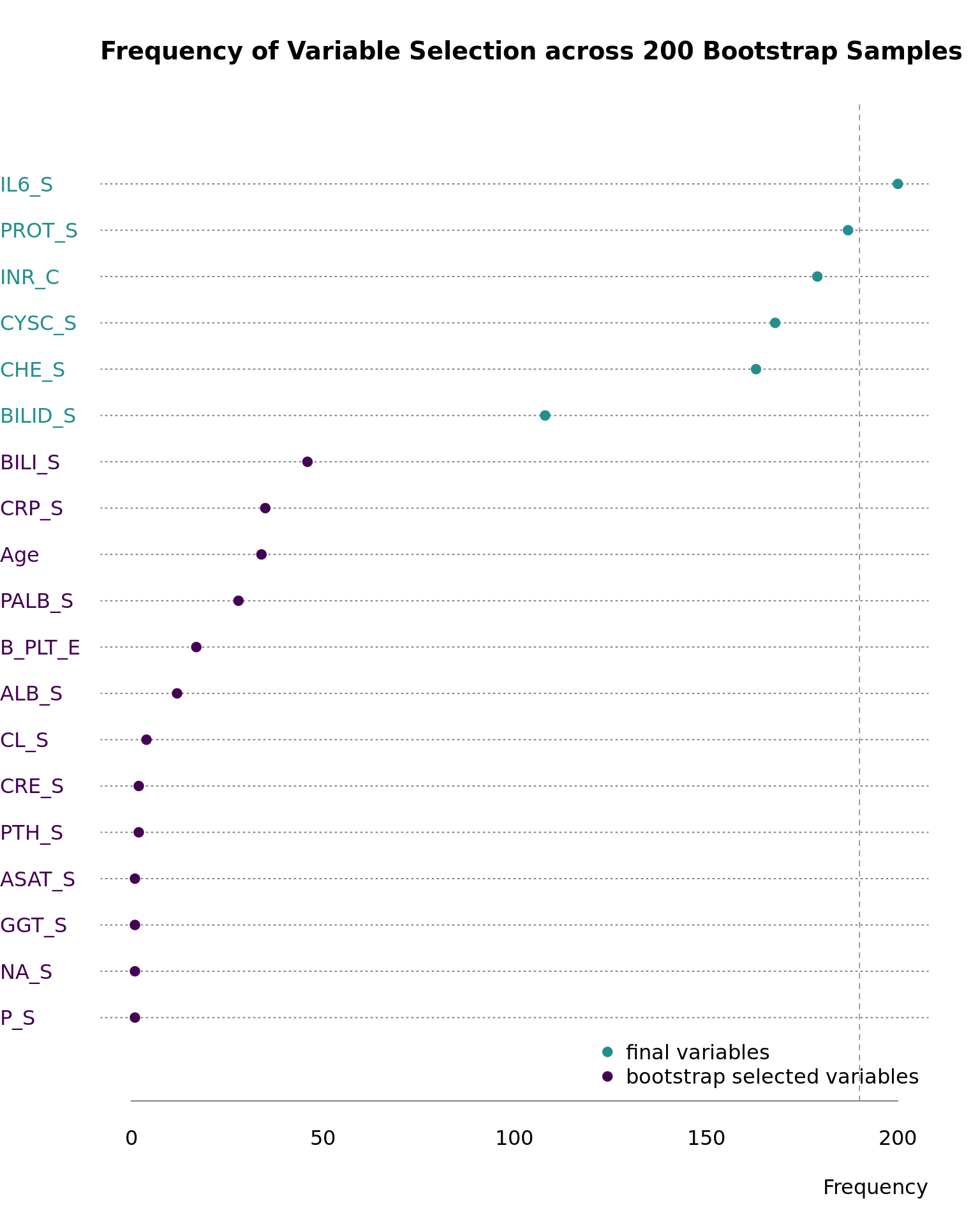
Figure 6.1: Variable importance by frequency of bootstrap selections.
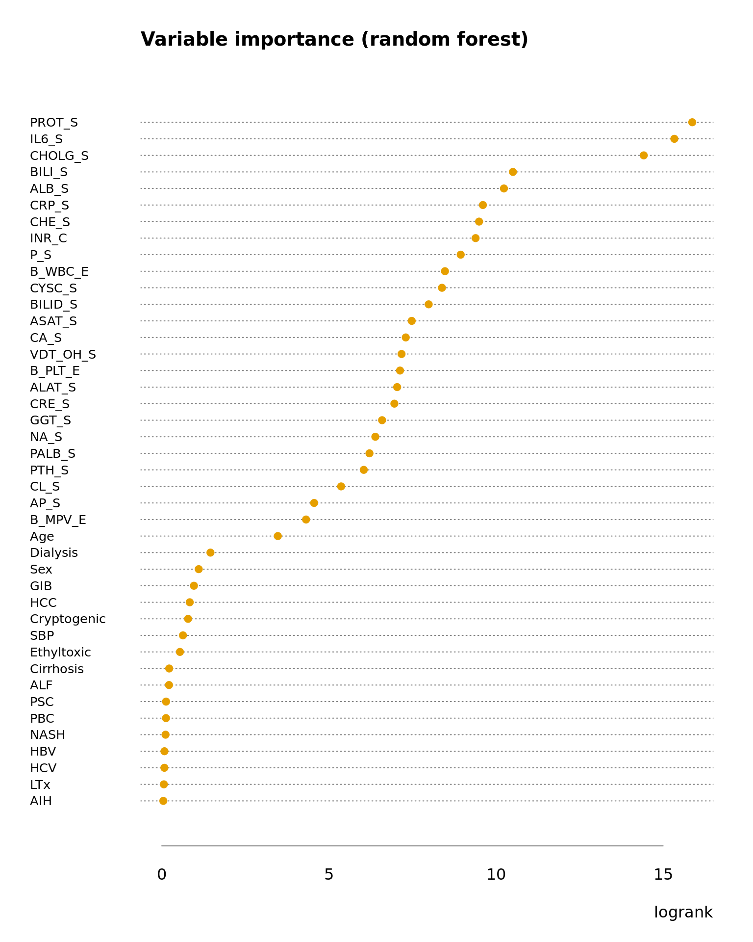
Figure 6.2: Variable importance by logrank in random forest.
7 References
sessionInfo()R version 4.2.0 (2022-04-22)
Platform: x86_64-unknown-linux-gnu (64-bit)
Matrix products: default
BLAS/LAPACK: /gnu/store/ras6dprsw3wm3swk23jjp8ww5dwxj333-openblas-0.3.18/lib/libopenblasp-r0.3.18.so
locale:
[1] LC_CTYPE=en_US.UTF-8 LC_NUMERIC=C
[3] LC_TIME=en_US.UTF-8 LC_COLLATE=en_US.UTF-8
[5] LC_MONETARY=en_US.UTF-8 LC_MESSAGES=en_US.UTF-8
[7] LC_PAPER=en_US.UTF-8 LC_NAME=C
[9] LC_ADDRESS=C LC_TELEPHONE=C
[11] LC_MEASUREMENT=en_US.UTF-8 LC_IDENTIFICATION=C
attached base packages:
[1] stats graphics grDevices utils datasets methods base
other attached packages:
[1] ggplot2_3.3.6 viridis_0.6.2 viridisLite_0.4.0 mlr3viz_0.5.9
[5] mlr3proba_0.4.11 mlr3misc_0.10.0 mlr3_0.13.3 targets_0.12.1
[9] data.table_1.14.2 ameld_0.0.31 survival_3.3-1 glmnet_4.1-4
[13] Matrix_1.4-1
loaded via a namespace (and not attached):
[1] fs_1.5.2 bbotk_0.5.3 rprojroot_2.0.3
[4] numDeriv_2016.8-1.1 mlr3pipelines_0.4.1 tools_4.2.0
[7] backports_1.4.1 bslib_0.3.1 utf8_1.2.2
[10] R6_2.5.1 colorspace_2.0-3 withr_2.5.0
[13] tidyselect_1.1.2 gridExtra_2.3 processx_3.5.3
[16] compiler_4.2.0 git2r_0.30.1 cli_3.3.0
[19] ooplah_0.2.0 lgr_0.4.3 timeROC_0.4
[22] labeling_0.4.2 bookdown_0.26 sass_0.4.1
[25] scales_1.2.0 checkmate_2.1.0 mvtnorm_1.1-3
[28] pec_2022.05.04 callr_3.7.0 palmerpenguins_0.1.0
[31] mlr3tuning_0.13.1 stringr_1.4.0 digest_0.6.29
[34] mlr3extralearners_0.5.37 rmarkdown_2.14 param6_0.2.4
[37] paradox_0.9.0 set6_0.2.4 pkgconfig_2.0.3
[40] htmltools_0.5.2 parallelly_1.31.1 fastmap_1.1.0
[43] highr_0.9 rlang_1.0.2 shape_1.4.6
[46] jquerylib_0.1.4 generics_0.1.2 farver_2.1.0
[49] jsonlite_1.8.0 dplyr_1.0.9 magrittr_2.0.3
[52] Rcpp_1.0.8.3 munsell_0.5.0 fansi_1.0.3
[55] lifecycle_1.0.1 stringi_1.7.6 whisker_0.4
[58] yaml_2.3.5 grid_4.2.0 parallel_4.2.0
[61] dictionar6_0.1.3 listenv_0.8.0 promises_1.2.0.1
[64] crayon_1.5.1 lattice_0.20-45 splines_4.2.0
[67] timereg_2.0.2 knitr_1.39 ps_1.7.0
[70] pillar_1.7.0 igraph_1.3.1 uuid_1.1-0
[73] base64url_1.4 future.apply_1.9.0 codetools_0.2-18
[76] glue_1.6.2 evaluate_0.15 vctrs_0.4.1
[79] httpuv_1.6.5 foreach_1.5.2 distr6_1.6.9
[82] gtable_0.3.0 purrr_0.3.4 future_1.26.1
[85] xfun_0.31 prodlim_2019.11.13 later_1.3.0
[88] tibble_3.1.7 iterators_1.0.14 lava_1.6.10
[91] workflowr_1.7.0 globals_0.15.0 ellipsis_0.3.2